As many readers know, I retired on July 31, 2025. The shift has gone well. But after a decade-plus of sustained strategic and operational attention to Supply Chain Resilience suddenly abandoning this field seemed self-betraying and hypocritical.
I have continued to receive some media and former-client inquiries, especially on tariff-related impacts to Supply Chain Resilience. I also hear from old friends and colleagues, even the occasional competitor. So, on a more or less weekly basis I have published here about big-picture issues of demand-pull, supply disequilibria, and the behavior of complex adaptive networks.
Going forward my contributions here will be less frequent, even mostly absent
This is certainly not because Supply Chain Resilience is a less important or a less urgent issue. Global terms of trade have been turned upside down over the last nine months. The frequency and severity of natural disasters continue to accelerate. If anything, structural and systemic resilience of demand and supply networks has never been more vital for more enterprises and their hundreds of millions of customers.
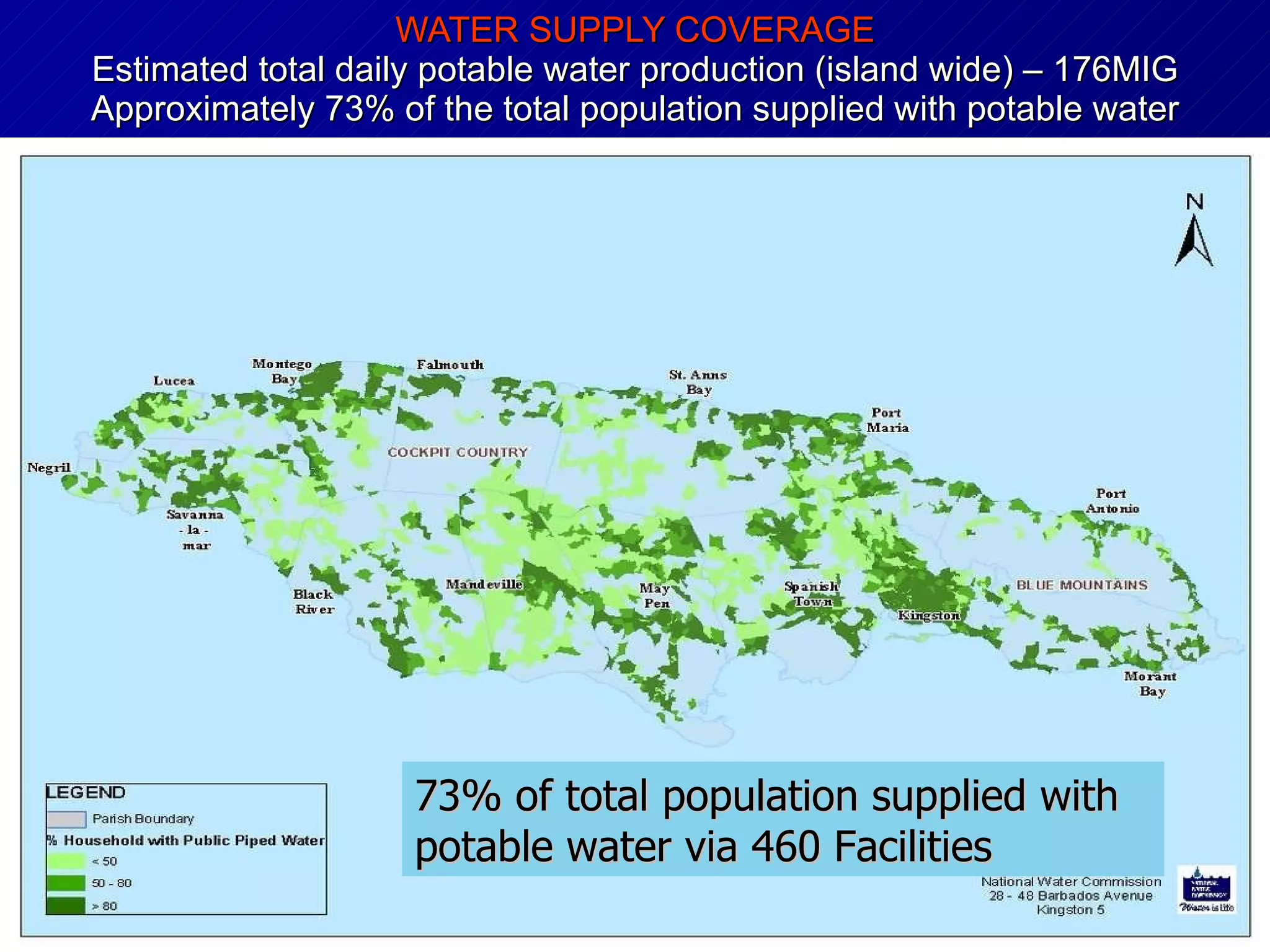
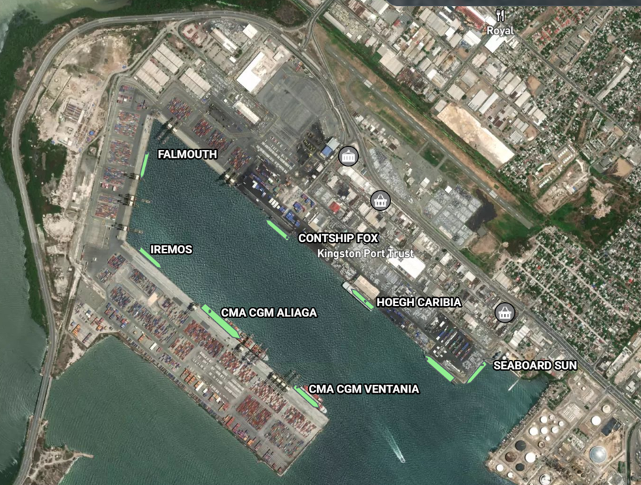
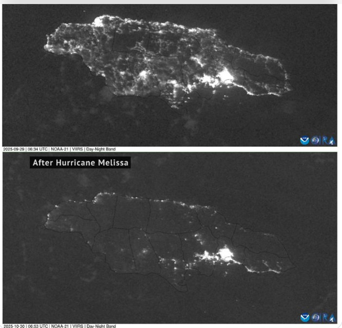
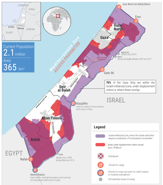
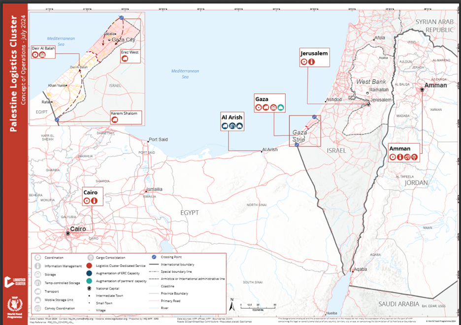
My step away mostly reflects three factors: First, since I am no longer invoicing, I am no longer motivated to engage in the same level of self-critical, self-correcting research and outreach that long characterized my professional life. As a result, my comparative value is gradually deteriorating. Better to stop before I make some huge neglectful mistake. Second, recent work related to post-hurricane recovery in Jamaica (and to a lesser degree, renewed relief supplies to Gaza) has delivered a strong sense that core principles of Supply Chain Resilience have been validated and should be well known, even obvious. So, especially when combined with the first factor it is better to step away from the game while I am emotionally/intellectually ahead. Third, I am enjoying my post-retirement priorities and want to invest even more there. Entirely self-centered, I realize. Retirees and two-year-olds can share several tendencies.
At some point, here or somewhere, I will probably write something more on tariff policy and Supply Chain Resilience. Once we see what the Supreme Court decides on presidential tariff authorities (here and here and here) and we see how the President responds, I may feel the need to close my own loop. Right now I expect this President to one way or another pursue the same tariff objectives I outlined on April 5 . (This September explanation is also relevant.) The goals and even the highest level strategies are likely to remain consistent. What tactics will be deployed depends on what specific authorities the Supreme Court confirms and available alternatives.
But however this case is decided and wherever the next major disaster strikes, I am happily fading away. Thank you for your interest in Supply Chain Resilience, your patience with me, and a wonderful flow of interesting questions and comments.